writings - Learning to rank with Multiple Objectives

MOO - The What, The Why & The How.

After that long detour, let’s now look into Multiple Objective Optimisation applied to Ranking problem within a marketplace setting involving multiple stakeholders. Let’s do so with a simple illustrative example that involves similar item recommendations. Specifically, let’s understand Why this is needed first.

Picture this, A User has browsed and explored a bunch of different red shirts they are planning to buy, and on one such open tab we’ve got a shirt that they are closely examining. Now, the recommendation system in the backend is also generating a bunch of similar shirts that they might be interested to explore. Let’s say the recommendation system is optimising for two different objectives - firstly, to show relevant and personalised shirts similar to their style based on interaction history. Secondly, the platform also wants to make sure it’s making a good profit on each sales that the recommendation system generates or leads to. Hence, they would also want to promote shirts with good porfit margin. How would we do this?

Let’s start by defining our objectives:

Objective I	Objective II
Personalisation	Price Margin

Let’s also say the item options available to us to be displayed (let’s focus on finding the top-1 item at the moment.) if plotted on a graph look something like this:

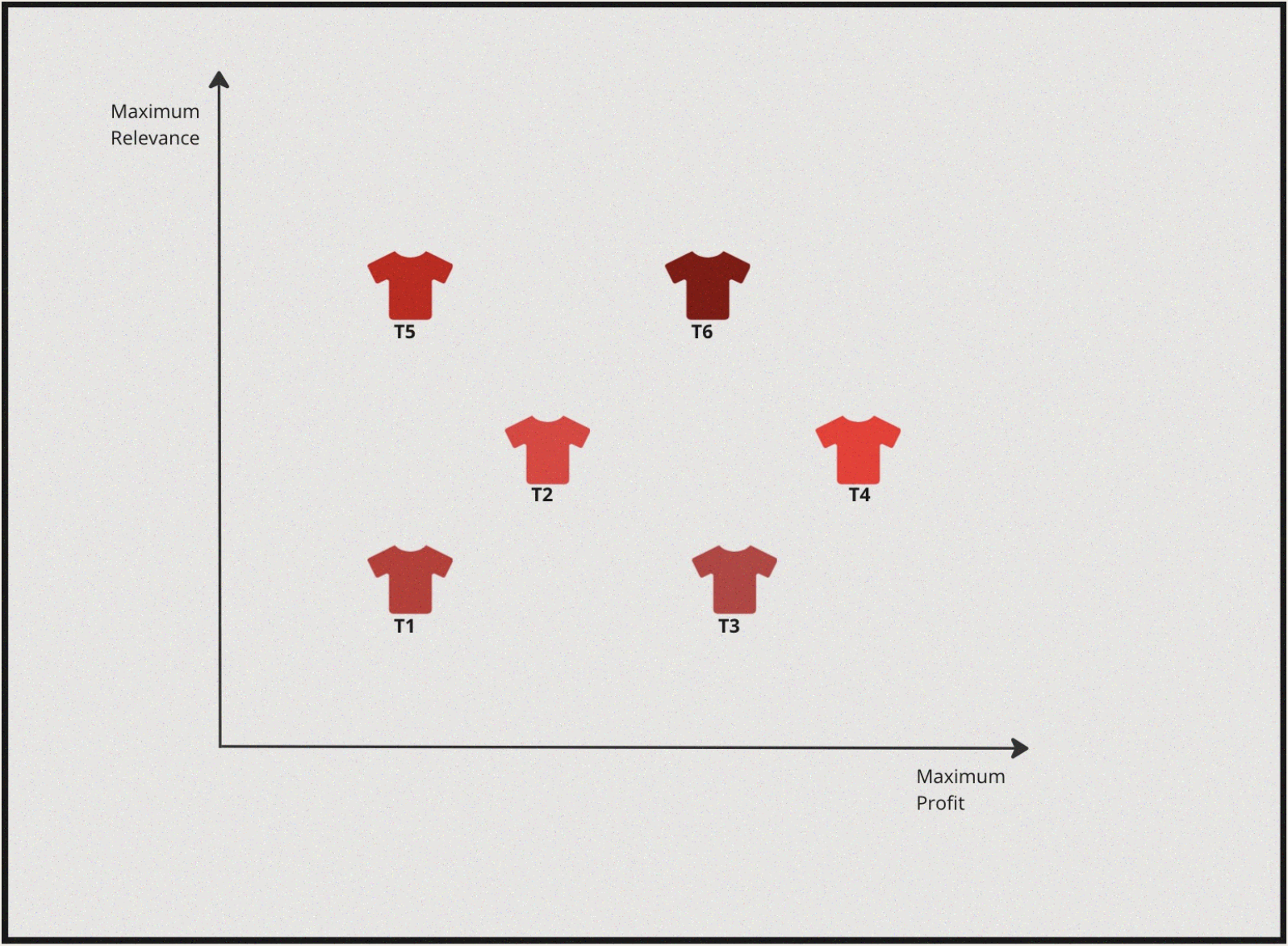
Now, essentially we want to maximise profit margin but also we want to maximise for highly personalised & relevant shirt. If we were to solve this from a lens of single objectve optimisation two scenarios would arise:

Case-I: Applying 1D Optimisation to objective I followed by optimising for objective II, i.e First we can find Highly Personalised shirts and then search for the shirt that also provides maximum margin.
Case-II: Applying 1D Optimisation to objective II followed by optimising for objective I, i.e First we can find High Profit margin shirts and then search for the ones which are also Highly Personalised & relevant for the user’s style.

For a simple and better understanding of the concept, assume that someone is trying to find the best red shirt from both the perspectives manually in a physical store, and let’s further also assume its a dark room.

Case I : Highly Personalised & High Profit margin

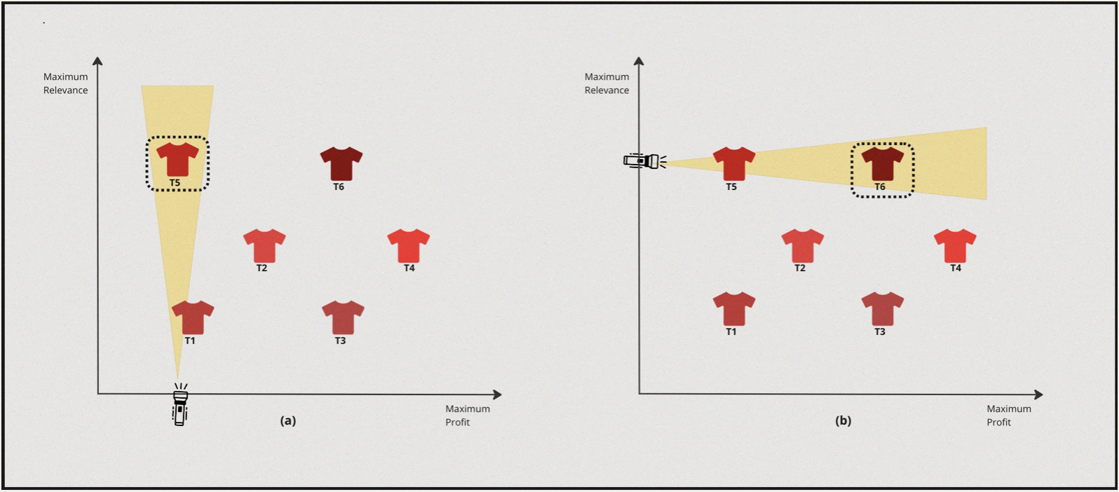
So, in this case the solver turns the torch on towards the relevance axis and discovers \(T5\) as the most suitable candidate.
Now from this point the solver turns towards the profit axis and turns the torch on and discovers \(T6\).

Case II : High Profit margin & High Personalisation

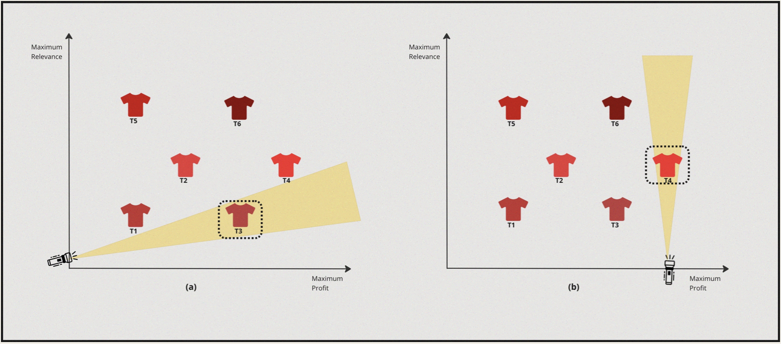
In this case the solver turns the torch on towards the profit axis and discovers \(T3\) as the best candidate.
Now from this point the solver turns towards the relevance axis and turns the torch on and discovers \(T4\).

What do we have as of now:

Process	1st Optimization Objective	2nd Optimization Objective	Optimal Solution
1	Personalisation	Profit Margin	\(T6\)
2	Profit Margin	Personalisation	\(T4\)

So, that seems odd. There are multiple solutions. Depending on what we want to achieve- If we want to optimize for both objectives and find the best solution, Going about in the above method is not the best way. Instead, we need to optimize to find solutions for both objectives collectively. The set of optimization methods that enables this is called Multiple Objective Optimization.

Let’s define what MOO is & try to understand some other key concepts associated with it.

Basic Concepts - Defining the MOO Problem, Pareto Optimum & Pareto Frontier

MOO: Optimization that involves identifying the values of decision (or free) variables that generate the maximum or minimum of one or more objectives. In most engineering problems, there may exist multiple, conflicting objectives and solving the optimization problems is not trivial or may not be even feasible sometimes. One way to formulate this is as follows:

Given \(m\) inequality constraints & \(p\) equality constraints identify a vector \(\bar{x}^*_n = [x^*_1, x^*_2,...,x^*_n]^T\) that optimizes

\[\bar{f}_k(\bar{x}_n) = [o_1(\bar{x}_n), o_2(\bar{x}_n),..., o_k(\bar{x}_n)]^T\]

such that

\[g_i(\bar{x}_n) ≥ 0, i = 1, 2, . . . , m\]

\[h_i( \bar{x}_n) = 0, i = 1, 2, . . . , p\]

where \(\bar{x}_n = [x_1, x_2, . . . , x_n]^T\) is a vector of \(n\) decision variables. The constraints determine the “feasible region” \(F\) and any point \(\bar{x}_n ∈ F\) gives a “feasible solution” where \(g_i( \bar{x}_n)\) and \(h_i( \bar{x}_n)\) are the constraints imposed on decision variables. The vector function \(\bar{f}_k(\bar{x}_n)\) above is a set of \(k\) objective functions, \(o_i(\bar{x}_n)\) for \(i = 1, · · · , k\), representing k non-commensurable criteria.

Pareto Optimum: A point \(\bar{x}^∗\) is “Pareto optimal” (for minimisation task) if the following holds for every \(\bar{x}_n ∈ F\)

\[\bar{f}_k(\bar{x}^*_n) ≤ \bar{f}_k( \bar{x}_n)\]

where \(\bar{f}_k(\bar{x}_n) = [o_1(\bar{x}_n), o_2(\bar{x}_n),..., o_k(\bar{x}_n)]^T\), \(\bar{f}^*_k(\bar{x}^*_n) = [o_1(\bar{x}^*_n), o_2(\bar{x}^*_n),..., o_k(\bar{x}^*_n)]^T\)

Pareto optimality gives a set of nondominated solutions. A feasible solution \(x\) is called “weakly nondominated” if there is no \(y ∈ F\) , such that \(o_i(y) < o_i(x)\) for all \(i = 1, 2, ..., k\). This means that there is no other feasible solution that can strictly dominate \(x\). A feasible solution \(x\) is called “strongly nondominated” if there is no \(y ∈ F\) , such that \(o_i(y) ≤ o_i(x)\) for all \(i = 1, 2, ...k\), and \(o_i(y) < o_i(x)\) for at least one \(i\). This means that there is no other feasible solution that can improve some objectives without worsening at least one other objective. If \(x\) is “strongly nondominated”, it is also “weakly nondominated”.

Pareto Frontier: A set (of feasible solutions) that is Pareto efficient is called the Pareto frontier, Pareto set, or Pareto front. The optimal solutions can be determined based on the tradeoffs within this set based on a designer’s decisions for acceptable performance.