A Quick Recap on modern recsys
Add brief intro about modern system here.
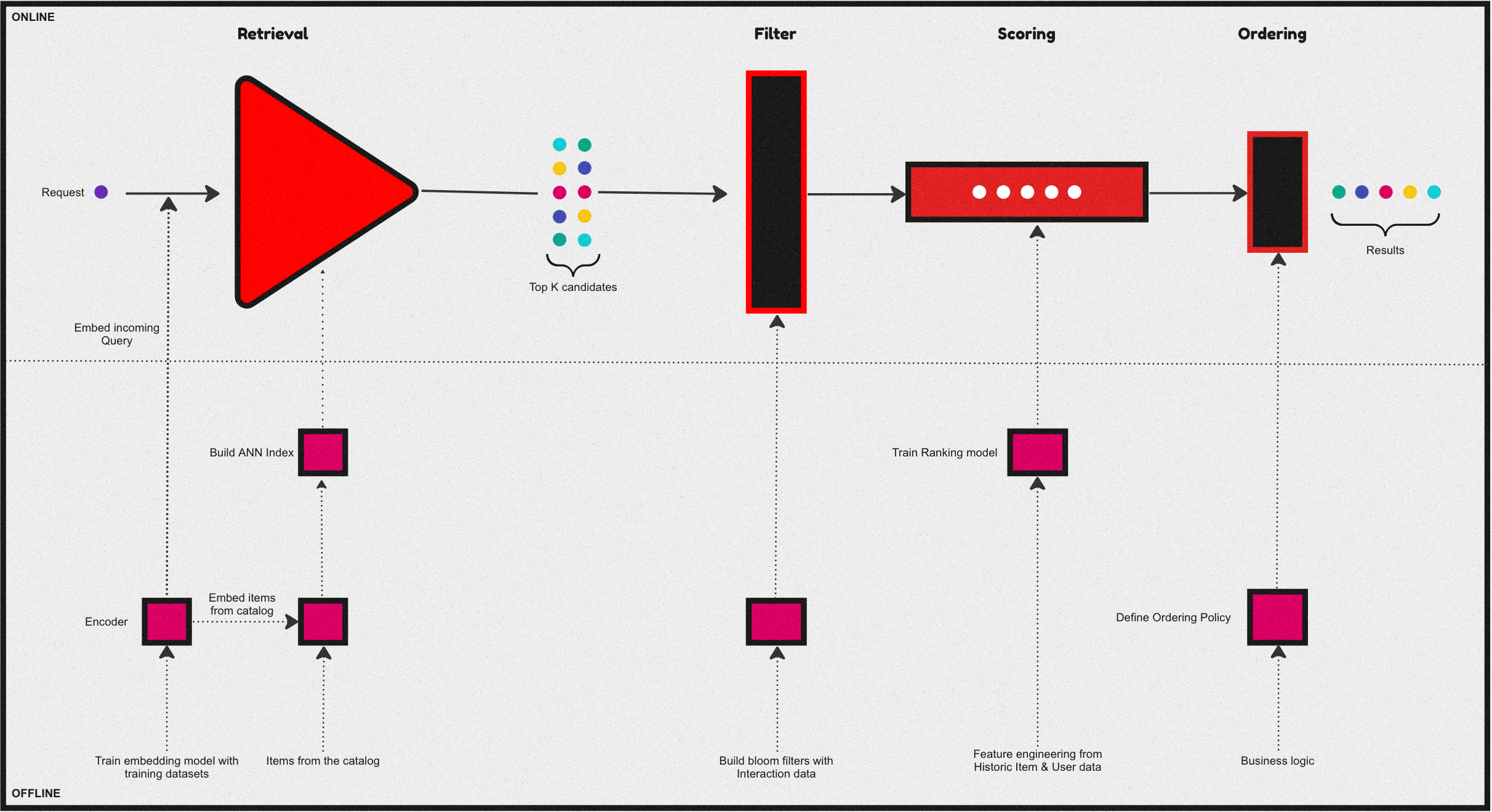
Over the past few years, a common and central design pattern has emerged around how most industrial recommendation systems are designed. If one were to summarise this design pattern, it would appear as described in the above figure - consisting of 4 stages. Let us take a brief look at the functionality of these four stages:
Candidate retrieval
The Retrieval & filtering stages usually are collectively referred to as candidate generation. A fast but coarse step which narrows down the search space of items from millions of candidates for a given query to something in the order of 100s.
Often this is achieved by an initial retrieval with some form of matching between the query and the catalog.Usually, via an ANN, Graph-based approach, or some form of a decision tree. Followed by a filtering stage, where invalid candidates are removed from the initial retrieval before passing on to the next stages.
Ranking
At this phase, we further narrow the initial set of items into a much smaller list to be presented to the user. Which is a slow but more precise operation - this stage is usually modeled as an LTR or a classification task. Further, sometimes it’s followed by an ordering stage which handles various business logic to reorder/sort the final list of items. Some common examples of this business logic include: organizing recommendations to fit genre distributions in streaming services or promoting specific segments of sellers as in the case of e-commerce.
A Quick Recap on Learning to Rank
Learning to rank (LTR) refers to a class of ML techniques for training a model to solve the task of ranking a set of items. Usually, this is formulated as a supervised or sometimes semi-supervised task.
Generally, this means we try to learn a function \(f(q, D)\) given a query \(q\) & a list of documents \(D\) to predict the order/rank of the documents within this list. Depending on how the loss function is formulated in the underlying task, any LTR algorithm can be classified into 3 distinct categories:
- Pointwise method
- Pairwise method
- Listwise method
Ranking Task
Given a query \(q\), and a set of \(n\) documents \(D=d_1,d_2,...,dn\), we’d like to learn a function \(f\) such that \(f(q, D)\) will predict the relevance of any given document associated with a query.
Pointwise method
In pointwise method, the above ranking task is re-formulated as a standard classification/regression task. The function to be learned \(f(q, D)\) is simplified as \(f(q, d_i)\) i.e the relevance of each document given a query is scored independently.
For instance, if we have two queries associated with 2 and 3 resulting matched documents:
- \(q_1 \to d_1, d_2\)
- \(q_2 \to d_3, d_4, d_5\)
Then the training data \(x_i\) in a pointwise method will essentially be every query-document pair as follows:
- \(x_1 : q_1, d_1\)
- \(x_2 : q_1, d_2\)
- \(x_3 : q_2, d_3\)
- \(x_4 : q_2, d_4\)
- \(x_5 : q_2, d_5\)
Since each document is scored independently with the absolute relevance as the target label, the task is no different from any standard classification or regression task. As such any standard ml algorithms can be leveraged in this setting.
Pairwise method
In pairwise method, the goal is to learn a pointwise scoring function \(f(q, d_i)\) similar to a pointwise formulation. However, the key difference arises in how the training data is consructed - where we take pairs of documents within the same query as training samples.
- \(x_1 \to q_1, (d_1, d_2)\)
- \(x_2 \to q_1, (d_3, d_4)\)
- \(x_3 \to q_1, (d_3, d_5)\)
- \(x_4 \to q_1, (d_4, d_5)\)
In this setting, a new set of pairwise binary labels are derived, by comapring the individual relevance score in each pair. For example, given the first query \(q_1\), if \(y_1==\) (i.e.. an irrelevant document) for \(d_1\) & \(y_2=3\) (i.e.. a Highly relevant document) for \(d_2\) then we can create a new label \(y_1<y_2\) for the pair of docs \((d_1, d_2)\) - by doing so we have essentially converted this back to a binary classification task again.
Now in order to learn the function \(f(q, d_i)\) which is still pointwise, but in a pairwise manner, we model the difference in scores probablistically as follows:
\[P(i>j) \equiv \frac{1}{1+exp^{-(s_i - s_j)}}\]
i.e, if document \(i\) is better matched than document \(j\) (denoted as \(i>j\)), then the probability of the scoring function to have scored \(f(q, d_i) = S_i\) should be close to 1. In other words, the model is trying to learn, given a query, how to score a pair of documents such that a more relevant document would be scored higher.
Listwise method
Listwise methods, solve the problem of ranking by learning to score the entire list jointly and they do so via two main sub techniques:
- Direct optimization of IR measures such as NDCG.(Eg: SoftRank, AdaRank).
- Minimize a loss function that is defined based on understanding the unique properties of the kind of ranking you are trying to achieve. (E.g. ListNet, ListMLE).
Let’s do a quick review of one of these approaches:
Consider ListNet, Which is based on the concept of permutation probability of a list of items. In this case we assume there is a pointwise scoring function \(f(q,di)\) used to score and rank a given list of items. But instead of modeling the probability as a pairwise comparison using scoring difference, we model the probability of the entire list of results. In this setting our documents and query dataset would appear like this:
- \(x_1 : q_1, (d_1, d_2)\)
- \(x_2 : q_2, (d_3, d_4, d_5)\)
First let’s look at the Permutation probability. Let’s denote \(π\) as a specific permutation of a given list of length \(n\), \(\Theta (s_i) = f(q, d_i)\) as any increasing function of scoring \(s_i\) given a query \(q\) and a document \(i\). The probability of having a permutation \(π\) can be written as follows:
\[P(\pi) = \prod_{i=1}^n \frac{\phi(s_i)}{\sum_{k=i}^n\phi(s_k)}\]
To illustrate consider a list of 3 items, then the probability of returning the permutation \(s_1\),\(s_2\),\(s_3\) is calculated as follows:
\[P(\pi = \{s_1, s_2, s_3\}) = \frac{\phi(s_1)}{\phi(s_1) + \phi(s_2) + \phi(s_3)} \cdot \frac{\phi(s_2)}{\phi(s_2) + \phi(s_3)} \cdot \frac{\phi(s_3)}{\phi(s_3)}\]
Due to computational complexity, ListNet simplies the problem by looking at only the top-one probability of a given item. The top-one probability of object i equals the sum of the permutation probabilities of permutations in which object i is ranked on the top. Indeed, the top-one probability of object i can be written as:
\[P(i) = \frac{\phi(s_i)}{\sum_{k=1}^n \phi(s_k)}\]
Given any two list of items represented by top-one probabilities, we can now measure the difference between them using cross entropy. Then we can use an ml algorithm which minimises that cross entropy. The choice of function \(ϕ(⋅)\), can be as simple as just an exponential function. When \(ϕ(⋅)\) is expotential and the list length is two, the solution basically reduces to a pairwise method as described earlier.
With that brief introduction out of the way, let’s also quickly look at the advantages and disadvantages of each of these approaches:
| Method | Advantages | Disadvantages |
|---|---|---|
| Pointwise |
|
|
| Pairwise |
|
|
| Listwise |
|
|